Flow Matching for Generative Modeling

Yaron Lipman, Ricky T. Q. Chen, Heli Ben-Hamu, Maximilian Nickel, Matt Le ICLR 2023

Continuous-time normalizing flows are general w.r.t. representing arbitrary probability paths (compared to diffusion, which is confined to Gaussianity) but hasn’t been tractable (unlike diffusion, which indirectly define a target probability path via a noising process). Here, we introduce a new objective, flow matching, which matches a target time-conditional PDF via a vector field that generates it. To derive a target PDF given only samples of the data distribution, we have to use conditional probabilities, basically Gaussian bumps around each datapoint (but could be other). We can then write a simpler conditional flow matching objective (which has the same gradients / solutions) which relies on first sampling $x_1 \sim q$ and then $x \sim p_t(x|x_1)$. All that’s left is to specify a flow (analogous to a noising process in diffusion) via $\mu_t(x)$ and $\sigma_t(x)$; choosing these corresponding to a normal distribution yields diffusion; choosing these to vary linearly w/ time yields OT (the quicker and empirically better method).

Background, motivations

Continuous (time) normalizing flows are more general than diffusion models, except existing methods to train them are too expensive or biased. Want this generality as well as efficiency. Currently, diffusion models are the only class of CNFs that can be efficiently trained, which is why everyone uses them despite being limited to certain distributions, namely Gaussians. Diffusion gets around these problems by indirectly¹ defining a target probability path via the noising process.

Also look at how concurrent works derived, what’s general principle and what are modifications one might make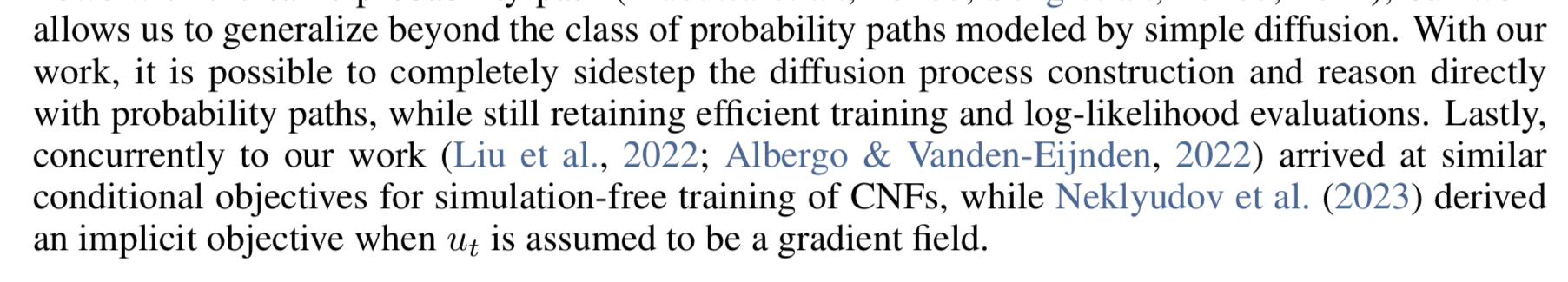

Continuous normalizing flows

Define a probability density path $p$ and a time-dependent vector field $v_t$. Define a flow $\phi_t$ as

\[\phi_{0}(x)=x; \frac{d}{dt}\phi_{t}(x) = v_t(\phi_t(x))\]

$v_{t}(x;\theta)$ is generally modeled with a NN and so the flow is defined indirectly through this vector field. $p$ is tied in via the push-forward operator (or change of variables)², which I won’t try to understand now. We can then say that $v_t$ generates probability path $p$ if $\phi$ and $p$ are related by the push-forward equation. The upshot is that the flow $\phi$ reshapes a simple probability distribution $p_0$ to a more complex one $p_1$ similar to the diffusion framework.

Flow Matching

We have samples drawn from a data distribution: $x \sim q(x_1)$ Flow matching objective: given a target density $p_t(x)$ and the vector field that generates it $u_t(x)$³, fit $v_{t}(x;\theta)$ to match the target flow.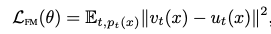 $t \sim U[0,1]$ and $x \sim p_t(x)$.

The obvious question is: how do we get $p_{t}(x)$ and $u_{t}(x)$ from $q$? Naively, we cannot. We’ll see that we can define them per-sample, which matches the fact that we can only access $q_1(x_1)$ through samples.

Conditional probability paths

Ultimately, we would like to get $p_{t}(x)$ and $u_{t}(x)$ from samples of $q$.

Given some data sample $x_{1}\sim q_1(x)$, let’s define conditional probabilities, $$p_t(x	x_1)$and$p_0(x	x_1)$with the restriction that the latter must equal the noise distribution$p_0(x)$. We will design$p_1(x	x_1)$to be a distribution concentrated around$x_1$such as a Gaussian with small variance. Combined across all datapoints, this will give a mixture distribution that closely approximates$q$$.
We can marginalize over $q$ as $$p_{t}(x) = \int p_{t}(x	x_{1})\cdot q(x_1)dx_1$. Note that for$t=1$,$p$should match$q$pretty closely. We can also define a marginal vector field$u_t(x)$though the derivation isn’t straightforward/obvious; this generates the marginal$p_t(x)$$. Importantly, this tells us that we can just define conditional vector fields and use this to get the marginal vector field. (Thm. 1)

However, the marginalization integrals are still intractable to compute.

Conditional flow matching

Instead, we’ll define a simpler objective. This shifts the burden to being able to (efficiently) sample from $p_t(x|x_1)$ and compute $u_t(x|x_1)$. This is easier b/c per-sample⁴. It turns out that this objective has the same gradients as our original flow matching objective, ergo they are equivalent. (Thm. 2)[[ ]]

Constructing conditional probability paths and vector fields

Will only consider Gaussian paths here, but can do any (continuous) distribution you’d like. We can define $p_0(x|x_1) = \mathcal{N}(0, 1)$ and $p_1(x|x_1) = \mathcal{N}(x_1, \sigma_{min})$.

Now we want a vector field that will generate a path between these two distributions. This vector field (and path, I believe) is generally not well or pre-specified; an infinite number of vector fields can generate a given probability path⁵. We choose to use the simplest⁶ flow, $\psi_t(x|x_1) = \sigma_t(x_1)\cdot x + \mu_t(x_1)$. The interpretation is that for $x \sim \mathcal{N}(0,1)$, this flow maps to the distribution $\mathcal{N}(\mu_t(x_1), \sigma_t(x_1))$. This seems analogous to the noising distribution in diffusion. Below equation confirms this: We can also just solve for $u$ then, because $\psi$ is simple and invertible: (Thm. 3)

Fitting other frameworks into flow matching

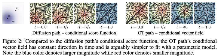
Notice how for OT, the vector field is always centered around the datapoint $x_1$, and the magnitude simply increases over time — indicative of linear interpolation btwn the starting point and $x_1$.

In contrast, the diffusion score function points to different points along the trajectory between the start and $x_1$ at different time steps, only settling onto $x_1$ at the end. This seems obviously worse in practice. What does this actually mean / why does this happen? → I think it’s b/c the perspective is how do I get from one timestep to the next, and each timestep defines $x_t$, and so we’re trying to get to that distribution, and so always taking something like $\nabla\log p_t(x_t|x_{t-1})$. This is different from e.g., $\nabla\log p(x_1|x_{t-1})$. This is because at each step, the score model is estimating the local denoising direction (because noise is added sequentially, locally too). Diffusion is more flexible than e.g., optimal transport⁷ because there’s an overparameterized network steering across the whole probability landscape decomposed into many steps (high complexity NN thus can construct high complexity distributions). Flow matching innovated on OT by using a conditional form in which OT happens per datapoint⁸ (instead of whole distribution) and is parameterized by a conditional vector field (which when fit over many datapoints, again can learn a complex probability landscape). This vector field is still time-dependent in the FM-OT case, but the directions are closer to being the same across timesteps, w/ magnitude increasing (which is consistent with OT linearly interpolating) — of course, not exact when we zoom out from the single datapoint case, as the vector fields are parameterized NNs fit in expectation over all datapoints on the conditional flow matching objective. ^3953ec

Gaussian diffusion

Can write diffusion processes (both variance-exploding and variance-preserving) as $p_t(x)$, which via Thm 3, allows us to write $u_t(x)$. The objective (flow matching) is still different from score matching — how to think about? — which may lead to different optimization performance. The authors report empirical improvements by using flow matching. There’s a remark about how these processes won’t actually reach true noise in finite time b/c coming from diffusion; I don’t understand. → This comes from Eq. 19, where we can see the denominator goes to 0 if $t=1$. More generally, we note (as shown in Figs 2, 3) that diffusion moves according to a time conditional grad log probability ($\nabla \log p_t(x)$), which because it’s time conditional, means only at t=1 will it match the true probability distribution’s gradient. I had been conceptualizing this as following gradient of probability distribution the whole time, but that’s actually much closer to what OT does. I should think about this more and reconcile the misunderstanding.

Optimal transport

Alternatively, we need not be bound to Gaussians. What if we linearly interpolate⁹ between $t=0$ and $t=1$? We can write simply:

\[\mu_t(x) = t\cdot x \;;\; \sigma_t(x) = 1-(1-\sigma_{\text{min}})\cdot t\]

OT is optimal in the somewhat straightforward sense, which is that it goes straight to $x_1$, whereas diffusion may overshoot and have to backtrack. Because OT path direction is constant in time, it should be an easier regression task.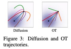

Experiments

Interestingly, evaluation time is one of the big gains over diffusion and similar generative models. For OT, interpretation is that it goes more directly. We notice empirically that OT begins showing patterns earlier on in the generative process than diffusion, which generally only shows them at the end¹⁰. FM diffusion is still faster than SM diffusion too—why? Also notes that sampling time may change (increase) during training for SM — this is because (see appendix Fig 10) they’re using a solver with a fixed tolerance, and apparently it takes SM more function evaluations to hit that tolerance, especially early on in training? This has to do with dopri5 solver¹¹ which gives adaptive step sizes. I’m not certain that this isn’t just construed; see Fig. 7 (left). However, FID gains (esp. w.r.t. NFE) do seem significant.

Connections

Probably relevant, good for contextualizing and tying together w/ diffusion framing: Diffusion Meets Flow Matching → This was alright, more on the practical side, a bit difficult for me to parse. Maybe worth returning to once I’ve been more inoculated in the diffusion / flow thinking. ^b833ff

Relevance

See Discrete Flow Models.

Footnotes

Indirect in the sense that a probability path is a time dependent PDF $p_t(x)$, but the forward noising process for diffusion only defines a transformation $$p(x_t

x_{t+1})$(adding noise) (adopting FM convention of noise @$t=0$and data @$t=1$$). Though this is still confusing looking at Eq. 16, since we have a form for a probability path (specified conditional on datapoints, still). I suspect this statement is in reference to the original diffusion framing, in which noising is thought of primarily as going from state to state, and not as the probability path it implies.

↩

I think this is similar to standard normalizing flow definitions that I’ve seen at some point. ↩
Do we actually have / know this? I thought we only got samples… ↩
I think analogous to diffusion in the sense that I just need to be able to noise each datapoint individually, not arbitrarily draw from the marginal noise distribution at time $t$. ↩
Though most of these are actions that the path is invariant to, leaving it unaltered. We’d like to avoid this b/c it burns compute to no effect. ↩
by what metric? ↩
Which requires explicit knowledge of both distributions to map between them, the full distribution. ↩
w.r.t. whole distribution, this is not an optimal transport mapping. And in practice, it will not be linear when sampling b/c you’re sampling globally, not interpolating to a specific datapoint. ↩
Argues that this is more natural. ↩
I think this is in accordance with noising schedules using in diffusion? If so, why don’t they just use noising schedules that noise more slowly close to the data and then faster when further? ↩
Impl. in torchdiffeq package, probably good to look into if going to work on this area. ↩

Given some data sample \(x_{1}\sim q_1(x)\), let’s define conditional probabilities, $$p_t(x	x_1)\(and\)p_0(x	x_1)\(with the restriction that the latter must equal the noise distribution\)p_0(x)\(. We will design\)p_1(x	x_1)\(to be a distribution concentrated around\)x_1\(such as a Gaussian with small variance. Combined across all datapoints, this will give a mixture distribution that closely approximates\)q$$.
We can marginalize over \(q\) as $$p_{t}(x) = \int p_{t}(x	x_{1})\cdot q(x_1)dx_1\(. Note that for\)t=1\(,\)p\(should match\)q\(pretty closely. We can also define a marginal vector field\)u_t(x)\(though the derivation isn’t straightforward/obvious; this generates the marginal\)p_t(x)$$. Importantly, this tells us that we can just define conditional vector fields and use this to get the marginal vector field. (Thm. 1)